Digital Signal Processing - Classification of Continuous Time Signals

Continuous time signals can be classified according to different conditions or operations performed on the signals.

Even and Odd Signals

Even Signal

A signal is said to be even if it satisfies the following condition;

x(−t)=x(t)$$$$

Time reversal of the signal does not imply any change on amplitude here. For example, consider the triangular wave shown below.

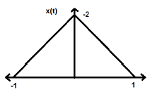
The triangular signal is an even signal. Since, it is symmetrical about Y-axis. We can say it is mirror image about Y-axis.

Consider another signal as shown in the figure below.

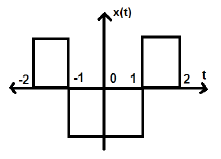
We can see that the above signal is even as it is symmetrical about Y-axis.

Odd Signal

A signal is said to be odd, if it satisfies the following condition

x(−t)=−x(t)$$$$

Here, both the time reversal and amplitude change takes place simultaneously.

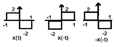
In the figure above, we can see a step signal x(t). To test whether it is an odd signal or not, first we do the time reversal i.e. x(-t) and the result is as shown in the figure. Then we reverse the amplitude of the resultant signal i.e. –x(-t) and we get the result as shown in figure.

If we compare the first and the third waveform, we can see that they are same, i.e. x(t)= -x(-t), which satisfies our criteria. Therefore, the above signal is an Odd signal.

Some important results related to even and odd signals are given below.

• Even × Even = Even
• Odd × Odd = Even
• Even × Odd = Odd
• Even ± Even = Even
• Odd ± Odd = Odd
• Even ± Odd = Neither even nor odd
• 
  

Representation of any signal into even or odd form

Some signals cannot be directly classified into even or odd type. These are represented as a combination of both even and odd signal.

x(t)→xe(t)+x0(t)$$$$

Where x_e(t) represents the even signal and x_o(t) represents the odd signal

xe(t)=[x(t)+x(−t)]2$$$$

And

x0(t)=[x(t)−x(−t)]2$$$$

Example

Find the even and odd parts of the signal x(n)=t+t2+t3

Solution − From reversing x(n), we get

x(−n)=−t+t2−t3$$$$

Now, according to formula, the even part

xe(t)=x(t)+x(−t)2$$$$

=[(t+t2+t3)+(−t+t2−t3)]2$$$$

=t2$$$$

Similarly, according to formula the odd part is

x0(t)=[x(t)−x(−t)]2$$$$

=[(t+t2+t3)−(−t+t2−t3)]2$$$$

=t+t3$$$$

Periodic and Non-Periodic Signals

Periodic Signals

Periodic signal repeats itself after certain interval of time. We can show this in equation form as −

x(t)=x(t)±nT$$$$

Where, n = an integer (1,2,3……)

T = Fundamental time period (FTP) ≠ 0 and ≠∞

Fundamental time period (FTP) is the smallest positive and fixed value of time for which signal is periodic.

A triangular signal is shown in the figure above of amplitude A. Here, the signal is repeating after every 1 sec. Therefore, we can say that the signal is periodic and its FTP is 1 sec.

Non-Periodic Signal

Simply, we can say, the signals, which are not periodic are non-periodic in nature. As obvious, these signals will not repeat themselves after any interval time.

Non-periodic signals do not follow a certain format; therefore, no particular mathematical equation can describe them.

Energy and Power Signals

A signal is said to be an Energy signal, if and only if, the total energy contained is finite and nonzero (0<E<∞). Therefore, for any energy type signal, the total normalized signal is finite and non-zero.

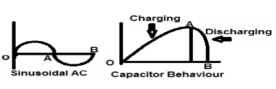
A sinusoidal AC current signal is a perfect example of Energy type signal because it is in positive half cycle in one case and then is negative in the next half cycle. Therefore, its average power becomes zero.

A lossless capacitor is also a perfect example of Energy type signal because when it is connected to a source it charges up to its optimum level and when the source is removed, it dissipates that equal amount of energy through a load and makes its average power to zero.

For any finite signal x(t) the energy can be symbolized as E and is written as;

E=∫+∞−∞x2(t)dt$$$$

Spectral density of energy type signals gives the amount of energy distributed at various frequency levels.

Power type Signals

A signal is said to be power type signal, if and only if, normalized average power is finite and non-zero i.e. (0<p<∞). For power type signal, normalized average power is finite and non-zero. Almost all the periodic signals are power signals and their average power is finite and non-zero.

In mathematical form, the power of a signal x(t) can be written as;

P=limT→∞1/T∫+T/2−T/2x2(t)dt$$$$

Difference between Energy and Power Signals

The following table summarizes the differences of Energy and Power Signals.

Power signal	Energy Signal
Practical periodic signals are power signals.	Non-periodic signals are energy signals.
Here, Normalized average power is finite and non-zero.	Here, total normalized energy is finite and non-zero.
Mathematically, P=limT→∞1/T∫+T/2−T/2x2(t)dt$$$$	Mathematically, E=∫+∞−∞x2(t)dt
Existence of these signals is infinite over time.	These signals exist for limited period of time.
Energy of power signal is infinite over infinite time.	Power of the energy signal is zero over infinite time.

Solved Examples

Example 1 − Find the Power of a signal z(t)=2cos(3Πt+30o)+4sin(3Π+30o)

Solution − The above two signals are orthogonal to each other because their frequency terms are identical to each other also they have same phase difference. So, total power will be the summation of individual powers.

Let z(t)=x(t)+y(t)

Where x(t)=2cos(3Πt+30o) and y(t)=4sin(3Π+30o)

Power of x(t)=222=2

Power of y(t)=422=8

Therefore, P(z)=p(x)+p(y)=2+8=10

Example 2 − Test whether the signal given x(t)=t2+jsintis conjugate or not?

Solution − Here, the real part being t² is even and odd part (imaginary) being sint$\sin t$ is odd. So the above signal is Conjugate signal.

Example 3 − Verify whether X(t)=sinωt is an odd signal or an even signal.

Solution − Given X(t)=sinωt

By time reversal, we will get sin(−ωt)

But we know that sin(−ϕ)=−sinϕ

Therefore,

sin(−ωt)=−sinωt$$$$

This is satisfying the condition for a signal to be odd. Therefore, sinωt$\sin \omega t$ is an odd signal.