Digital Signal Processing - Miscellaneous Signals

Image result for digital signal processor

There are other signals, which are a result of operation performed on them. Some common type of signals are discussed below.

Conjugate Signals

Signals, which satisfies the condition

x (t) = x * (- t)

are called conjugate signals.

Let

x (t) = a (t) + j b (t)

So,

x (- t) = a (- t) + j b (- t)

And

x * (- t) = a (- t) - j b (- t)

By Condition,

x (t) = x * (- t)

If we compare both the derived equations 1 and 2, we can see that the real part is even, whereas the imaginary part is odd. This is the condition for a signal to be a conjugate type.

Conjugate Anti-Symmetric Signals

Signals, which satisfy the condition

x (t) = - x * (- t)

are called conjugate anti-symmetric signal

Let

x (t) = a (t) + j b (t)

x (- t) = a (- t) + j b (- t)

And

x * (- t) = a (- t) - j b (- t)

- x * (- t) = - a (- t) + j b (- t)

By Condition

x (t) = - x * (- t)

Now, again compare, both the equations just as we did for conjugate signals. Here, we will find that the real part is odd and the imaginary part is even. This is the condition for a signal to become conjugate anti-symmetric type.

Example

Let the signal given be

x (t) = \sin t + j t^{2}

Here, the real part being

\sin t

is odd and the imaginary part being

t^{2}

is even. So, this signal can be classified as conjugate anti-symmetric signal.

Any function can be divided into two parts. One part being Conjugate symmetry and other part being conjugate anti-symmetric. So any signal x(t) can be written as

Where

x c s (t)

is conjugate symmetric signal and

x c a s (t)

is conjugate anti symmetric signal

x c s (t) = [ x ( t ) + x * ( - t ) ] 2

And

Half Wave Symmetric Signals

When a signal satisfies the condition

c x (t) = - x (t \pm (\frac{T_{0}}{2}))

, it is called half wave symmetric signal. Here, amplitude reversal and time shifting of the signal takes place by half time. For half wave symmetric signal, average value will be zero but this is not the case when the situation is reversed.

Image result for half wave symmetric signal

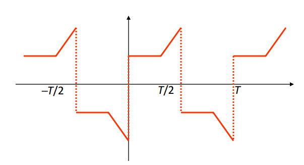
Consider a signal x(t) as shown in figure A above. The first step is to time shift the signal and make it

x [t - (\frac{T}{2})]

. So, the new signal is changed as shown in figure B. Next, we reverse the amplitude of the signal, i.e. make it

- x [t - (\frac{T}{2})]

as shown in the figure. Since, this signal repeats itself after half-time shifting and reversal of amplitude, it is a half wave symmetric signal.

Orthogonal Signal

Two signals x(t) and y(t) are said to be orthogonal if they satisfy the following two conditions.

Condition 1 −

\int_{- \infty}^{\infty} x (t) y (t) = 0

[for non-periodic signal]

Condition 2 −

\int x (t) y (t) = 0

[For periodic Signal]

The signals, which contain odd harmonics (3^rd, 5^th, 7^th ...etc.) and have different frequencies, are mutually orthogonal to each other.

In trigonometric type signals, sine functions and cosine functions are also orthogonal to each other; provided, they have same frequency and are in same phase. In the same manner DC (Direct current signals) and sinusoidal signals are also orthogonal to each other. If x(t) and y(t) are two orthogonal signals and

z (t) = x (t) + y (t)

then the power and energy of z(t) can be written as ;

P (z) = p (x) + p (y)

Example

Analyze the signal:

z (t) = 3 + 4 \sin (2 π t + 30^{0})

Here, the signal comprises of a DC signal and one sine function. So, by property this signal is an orthogonal signal and the two sub-signals in it are mutually orthogonal to each other.

Comments

Digital Signal Processing - Basic Continuous Time Signals

To test a system, generally, standard or basic signals are used. These signals are the basic building blocks for many complex signals. Hence, they play a very important role in the study of signals and systems. Unit Impulse or Delta Function A signal, which satisfies the condition, δ ( t ) = lim ϵ → ∞ x ( t ) δ ( t ) = lim ϵ → ∞ x ( t ) is known as unit impulse signal. This signal tends to infinity when t = 0 and tends to zero when t ≠ 0 such that the area under its curve is always equals to one. The delta function has zero amplitude everywhere except at t = 0. Properties of Unit Impulse Signal δ(t) is an even signal. δ(t) is an example of neither energy nor power (NENP) signal. Area of unit impulse signal can be written as; A = ∫ ∞ − ∞ δ ( t ) d t = ∫ ∞ − ∞ lim ϵ → 0 x ( t ) d t = lim ϵ → 0 ∫ ∞ − ∞ [ x ( t ) d t ] = 1 Weight or strength of the signal can be written as; y ( t ) = A δ ( t ) y ( t ) = A δ ( t ) Area of the weighted impulse signal can

Differential Equations - First Order: Bernoulli

In this section we are going to take a look at differential equations in the form, y ′ + p ( x ) y = q ( x ) y n y ′ + p ( x ) y = q ( x ) y n where p ( x ) p ( x ) and q ( x ) q ( x ) are continuous functions on the interval we’re working on and n n is a real number. Differential equations in this form are called Bernoulli Equations . First notice that if n = 0 n = 0 or n = 1 n = 1 then the equation is linear and we already know how to solve it in these cases. Therefore, in this section we’re going to be looking at solutions for values of n n other than these two. In order to solve these we’ll first divide the differential equation by y n y n to get, y − n y ′ + p ( x ) y 1 − n = q ( x ) y − n y ′ + p ( x ) y 1 − n = q ( x ) We are now going to use the substitution v = y 1 − n v = y 1 − n to convert this into a differential equation in terms of v v . As we’ll see this will lead to a differential equation that we can solve. We are going to have to be c

Differential Equations - Systems: Solutions

Now that we’ve got some of the basics out of the way for systems of differential equations it’s time to start thinking about how to solve a system of differential equations. We will start with the homogeneous system written in matrix form, → x ′ = A → x (1) (1) x → ′ = A x → where, A A is an n × n n × n matrix and → x x → is a vector whose components are the unknown functions in the system. Now, if we start with n = 1 n = 1 then the system reduces to a fairly simple linear (or separable) first order differential equation. x ′ = a x x ′ = a x and this has the following solution, x ( t ) = c e a t x ( t ) = c e a t So, let’s use this as a guide and for a general n n let’s see if → x ( t ) = → η e r t (2) (2) x → ( t ) = η → e r t will be a solution. Note that the only real difference here is that we let the constant in front of the exponential be a vector. All we need to do then is plug this into the differential equation and see what we get. First notice that

Calculus III - 3-Dimensional Space: Equations of Lines

In this section we need to take a look at the equation of a line in R 3 R 3 . As we saw in the previous section the equation y = m x + b y = m x + b does not describe a line in R 3 R 3 , instead it describes a plane. This doesn’t mean however that we can’t write down an equation for a line in 3-D space. We’re just going to need a new way of writing down the equation of a curve. So, before we get into the equations of lines we first need to briefly look at vector functions. We’re going to take a more in depth look at vector functions later. At this point all that we need to worry about is notational issues and how they can be used to give the equation of a curve. The best way to get an idea of what a vector function is and what its graph looks like is to look at an example. So, consider the following vector function. → r ( t ) = ⟨ t , 1 ⟩ r → ( t ) = ⟨ t , 1 ⟩ A vector function is a function that takes one or more variables, one in this case, and returns a vector. Note as we

Differential Equations - First Order: Modeling - i

We now move into one of the main applications of differential equations both in this class and in general. Modeling is the process of writing a differential equation to describe a physical situation. Almost all of the differential equations that you will use in your job (for the engineers out there in the audience) are there because somebody, at some time, modeled a situation to come up with the differential equation that you are using. This section is not intended to completely teach you how to go about modeling all physical situations. A whole course could be devoted to the subject of modeling and still not cover everything! This section is designed to introduce you to the process of modeling and show you what is involved in modeling. We will look at three different situations in this section : Mixing Problems, Population Problems, and Falling Objects. In all of these situations we will be forced to make assumptions that do not accurately depict reality in most cases, but wi

Differential Equations - Basic Concepts: Definitions

Differential Equation The first definition that we should cover should be that of differential equation . A differential equation is any equation which contains derivatives, either ordinary derivatives or partial derivatives. There is one differential equation that everybody probably knows, that is Newton’s Second Law of Motion. If an object of mass m m is moving with acceleration a a and being acted on with force F F then Newton’s Second Law tells us. F = m a (1) (1) F = m a To see that this is in fact a differential equation we need to rewrite it a little. First, remember that we can rewrite the acceleration, a a , in one of two ways. a = d v d t OR a = d 2 u d t 2 (2) (2) a = d v d t OR a = d 2 u d t 2 Where v v is the velocity of the object and u u is the position function of the object at any time t t . We should also remember at this point that the force, F F may also be a function of time, velocity, and/or position. So, with all these things in

Differential Equations - Partial: Summary of Separation of Variables

Throughout this chapter we’ve been talking about and solving partial differential equations using the method of separation of variables. However, the one thing that we’ve not really done is completely work an example from start to finish showing each and every step. Each partial differential equation that we solved made use somewhere of the fact that we’d done at least part of the problem in another section and so it makes some sense to have a quick summary of the method here. Also note that each of the partial differential equations only involved two variables. The method can often be extended out to more than two variables, but the work in those problems can be quite involved and so we didn’t cover any of that here. So with all of that out of the way here is a quick summary of the method of separation of variables for partial differential equations in two variables. Verify that the partial differential equation is linear and homogeneous. Verify that the boundary condi

Differential Equations - Systems: Repeated Eigenvalues - i

This is the final case that we need to take a look at. In this section we are going to look at solutions to the system, → x ′ = A → x x → ′ = A x → where the eigenvalues are repeated eigenvalues. Since we are going to be working with systems in which A A is a 2 × 2 2 × 2 matrix we will make that assumption from the start. So, the system will have a double eigenvalue, λ λ . This presents us with a problem. We want two linearly independent solutions so that we can form a general solution. However, with a double eigenvalue we will have only one, → x 1 = → η e λ t x → 1 = η → e λ t So, we need to come up with a second solution. Recall that when we looked at the double root case with the second order differential equations we ran into a similar problem. In that section we simply added a t t to the solution and were able to get a second solution. Let’s see if the same thing will work in this case as well. We’ll see if → x = t e λ t → η x → = t e λ t η → will also be a

Differential Equations - First Order: Modeling - ii

Example 4 A 50 kg object is shot from a cannon straight up with an initial velocity of 10m/s off a bridge that is 100 meters above the ground. If air resistance is given by 5 v v determine the velocity of the mass when it hits the ground. First, notice that when we say straight up, we really mean straight up, but in such a way that it will miss the bridge on the way back down. Here is a sketch of the situation. Notice the conventions that we set up for this problem. Since the vast majority of the motion will be in the downward direction we decided to assume that everything acting in the downward direction should be positive. Note that we also defined the “zero position” as the bridge, which makes the ground have a “position” of 100. Okay, if you think about it we actually have two situations here. The initial phase in which the mass is rising in the air and the second phase when the mass is on its way down. We will need to examine both situations and set up an IVP for

Robert Karamagi

Search This Blog

Calculus III - 3-Dimensional Space: Equations of Lines