
Calculus III - 3-Dimensional Space: Equations of Lines

In this section we need to take a look at the equation of a line in  R 3 R 3 . As we saw in the previous section the equation  y = m x + b y = m x + b  does not describe a line in  R 3 R 3 , instead it describes a plane. This doesn’t mean however that we can’t write down an equation for a line in 3-D space. We’re just going to need a new way of writing down the equation of a curve. So, before we get into the equations of lines we first need to briefly look at vector functions. We’re going to take a more in depth look at vector functions later. At this point all that we need to worry about is notational issues and how they can be used to give the equation of a curve. The best way to get an idea of what a vector function is and what its graph looks like is to look at an example. So, consider the following vector function. → r ( t ) = ⟨ t , 1 ⟩ r → ( t ) = ⟨ t , 1 ⟩ A vector function is a function that takes one or more variables, one in this case, and returns a...

Digital Signal Processing - Operations on Signals: Scaling

Image result for digital signal processor


Scaling of a signal means, a constant is multiplied with the time or amplitude of the signal.

Time Scaling

If a constant is multiplied to the time axis then it is known as Time scaling. This can be mathematically represented as;
 or  ; where α ≠ 0
So the y-axis being same, the x- axis magnitude decreases or increases according to the sign of the constant (whether positive or negative). Therefore, scaling can also be divided into two categories as discussed below.

Time Compression

Whenever alpha is greater than zero, the signal’s amplitude gets divided by alpha whereas the value of the Y-axis remains the same. This is known as Time Compression.

Example
Let us consider a signal x(t), which is shown as in figure below. Let us take the value of alpha as 2. So, y(t) will be x(2t), which is illustrated in the given figure.
Time Compression Example
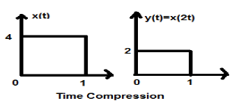
Clearly, we can see from the above figures that the time magnitude in y-axis remains the same but the amplitude in x-axis reduces from 4 to 2. Therefore, it is a case of Time Compression.
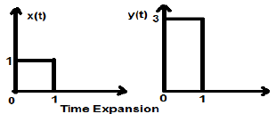
Time Expansion

When the time is divided by the constant alpha, the Y-axis magnitude of the signal get multiplied alpha times, keeping X-axis magnitude as it is. Therefore, this is called Time expansion type signal.
Example
Let us consider a square signal x(t), of magnitude 1. When we time scaled it by a constant 3, such that , then the signal’s amplitude gets modified by 3 times which is shown in the figure below.
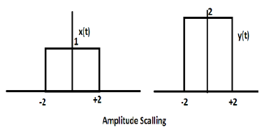
Time Expansion Example

Amplitude Scaling

Multiplication of a constant with the amplitude of the signal causes amplitude scaling. Depending upon the sign of the constant, it may be either amplitude scaling or attenuation. Let us consider a square wave signal x(t) = Π(t/4).
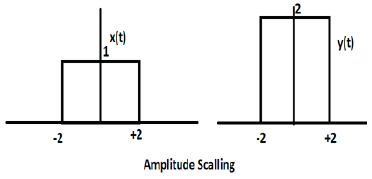
Suppose we define another function y(t) = 2 Π(t/4). In this case, value of y-axis will be doubled, keeping the time axis value as it is. The is illustrated in the figure given below.
Amplitude Scaling
Consider another square wave function defined as z(t) where z(t) = 0.5 Π(t/4). Here, amplitude of the function z(t) will be half of that of x(t) i.e. time axis remaining same, amplitude axis will be halved. This is illustrated by the figure given below.
Amplitude Attenuation

Comments

Popular posts from this blog

Digital Signal Processing - Basic Continuous Time Signals

To test a system, generally, standard or basic signals are used. These signals are the basic building blocks for many complex signals. Hence, they play a very important role in the study of signals and systems. Unit Impulse or Delta Function A signal, which satisfies the condition,   δ ( t ) = lim ϵ → ∞ x ( t ) δ ( t ) = lim ϵ → ∞ x ( t )   is known as unit impulse signal. This signal tends to infinity when t = 0 and tends to zero when t ≠ 0 such that the area under its curve is always equals to one. The delta function has zero amplitude everywhere except at t = 0. Properties of Unit Impulse Signal δ(t) is an even signal. δ(t) is an example of neither energy nor power (NENP) signal. Area of unit impulse signal can be written as; A = ∫ ∞ − ∞ δ ( t ) d t = ∫ ∞ − ∞ lim ϵ → 0 x ( t ) d t = lim ϵ → 0 ∫ ∞ − ∞ [ x ( t ) d t ] = 1 Weight or strength of the signal can be written as; y ( t ) = A δ ( t ) y ( t ) = A δ ( t ) Area of the weighted impulse s...

Differential Equations - First Order: Bernoulli

In this section we are going to take a look at differential equations in the form, y ′ + p ( x ) y = q ( x ) y n y ′ + p ( x ) y = q ( x ) y n where  p ( x ) p ( x )  and  q ( x ) q ( x )  are continuous functions on the interval we’re working on and  n n  is a real number. Differential equations in this form are called  Bernoulli Equations . First notice that if  n = 0 n = 0  or  n = 1 n = 1  then the equation is linear and we already know how to solve it in these cases. Therefore, in this section we’re going to be looking at solutions for values of  n n  other than these two. In order to solve these we’ll first divide the differential equation by  y n y n  to get, y − n y ′ + p ( x ) y 1 − n = q ( x ) y − n y ′ + p ( x ) y 1 − n = q ( x ) We are now going to use the substitution  v = y 1 − n v = y 1 − n  to convert this into a differential equation in terms of  v v . As we’ll see th...

Differential Equations - Systems: Solutions

Now that we’ve got some of the basics out of the way for systems of differential equations it’s time to start thinking about how to solve a system of differential equations. We will start with the homogeneous system written in matrix form, → x ′ = A → x (1) (1) x → ′ = A x → where,  A A  is an  n × n n × n  matrix and  → x x →  is a vector whose components are the unknown functions in the system. Now, if we start with  n = 1 n = 1 then the system reduces to a fairly simple linear (or separable) first order differential equation. x ′ = a x x ′ = a x and this has the following solution, x ( t ) = c e a t x ( t ) = c e a t So, let’s use this as a guide and for a general  n n  let’s see if → x ( t ) = → η e r t (2) (2) x → ( t ) = η → e r t will be a solution. Note that the only real difference here is that we let the constant in front of the exponential be a vector. All we need to do then is plug this into the d...

Digital Signal Processing - Miscellaneous Signals

There are other signals, which are a result of operation performed on them. Some common type of signals are discussed below. Conjugate Signals Signals, which satisfies the condition  x ( t ) = x ∗ ( − t ) are called conjugate signals. Let  x ( t ) = a ( t ) + j b ( t ) So,  x ( − t ) = a ( − t ) + j b ( − t ) And  x ∗ ( − t ) = a ( − t ) − j b ( − t ) By Condition,  x ( t ) = x ∗ ( − t ) If we compare both the derived equations 1 and 2, we can see that the real part is even, whereas the imaginary part is odd. This is the condition for a signal to be a conjugate type. Conjugate Anti-Symmetric Signals Signals, which satisfy the condition  x ( t ) = − x ∗ ( − t ) are called conjugate anti-symmetric signal Let  x ( t ) = a ( t ) + j b ( t ) So  x ( − t ) = a ( − t ) + j b ( − t ) And  x ∗ ( − t ) = a ( − t ) − j b ( − t ) − x ∗ ( − t ) = − a ( − t ) + j b ( − t ) By Condition  x ( t ) = − x ∗ ( − t ) ...

Calculus III - 3-Dimensional Space: Equations of Lines

In this section we need to take a look at the equation of a line in  R 3 R 3 . As we saw in the previous section the equation  y = m x + b y = m x + b  does not describe a line in  R 3 R 3 , instead it describes a plane. This doesn’t mean however that we can’t write down an equation for a line in 3-D space. We’re just going to need a new way of writing down the equation of a curve. So, before we get into the equations of lines we first need to briefly look at vector functions. We’re going to take a more in depth look at vector functions later. At this point all that we need to worry about is notational issues and how they can be used to give the equation of a curve. The best way to get an idea of what a vector function is and what its graph looks like is to look at an example. So, consider the following vector function. → r ( t ) = ⟨ t , 1 ⟩ r → ( t ) = ⟨ t , 1 ⟩ A vector function is a function that takes one or more variables, one in this case, and returns a...

Differential Equations - First Order: Modeling - i

We now move into one of the main applications of differential equations both in this class and in general. Modeling is the process of writing a differential equation to describe a physical situation. Almost all of the differential equations that you will use in your job (for the engineers out there in the audience) are there because somebody, at some time, modeled a situation to come up with the differential equation that you are using. This section is not intended to completely teach you how to go about modeling all physical situations. A whole course could be devoted to the subject of modeling and still not cover everything! This section is designed to introduce you to the process of modeling and show you what is involved in modeling. We will look at three different situations in this section : Mixing Problems, Population Problems, and Falling Objects. In all of these situations we will be forced to make assumptions that do not accurately depict reality in most cases, but wi...

Differential Equations - Basic Concepts: Definitions

Differential Equation The first definition that we should cover should be that of  differential equation . A differential equation is any equation which contains derivatives, either ordinary derivatives or partial derivatives. There is one differential equation that everybody probably knows, that is Newton’s Second Law of Motion. If an object of mass  m m  is moving with acceleration  a a  and being acted on with force  F F  then Newton’s Second Law tells us. F = m a (1) (1) F = m a To see that this is in fact a differential equation we need to rewrite it a little. First, remember that we can rewrite the acceleration,  a a , in one of two ways. a = d v d t OR a = d 2 u d t 2 (2) (2) a = d v d t OR a = d 2 u d t 2 Where  v v  is the velocity of the object and  u u  is the position function of the object at any time  t t . We should also remember at this point that the force,  F F  may also be a f...

Differential Equations - Second Order: Repeated Roots

In this section we will be looking at the last case for the constant coefficient, linear, homogeneous second order differential equations. In this case we want solutions to a y ′′ + b y ′ + c y = 0 a y ″ + b y ′ + c y = 0 where solutions to the characteristic equation a r 2 + b r + c = 0 a r 2 + b r + c = 0 are double roots  r 1 = r 2 = r r 1 = r 2 = r . This leads to a problem however. Recall that the solutions are y 1 ( t ) = e r 1 t = e r t y 2 ( t ) = e r 2 t = e r t y 1 ( t ) = e r 1 t = e r t y 2 ( t ) = e r 2 t = e r t These are the same solution and will NOT be “nice enough” to form a general solution. We do promise that we’ll define “nice enough” eventually! So, we can use the first solution, but we’re going to need a second solution. Before finding this second solution let’s take a little side trip. The reason for the side trip will be clear eventually. From the quadratic formula we know that the roots to the characteristic equation are, r 1 , 2 = ...

Differential Equations - Systems: Repeated Eigenvalues - i

This is the final case that we need to take a look at. In this section we are going to look at solutions to the system, → x ′ = A → x x → ′ = A x → where the eigenvalues are repeated eigenvalues. Since we are going to be working with systems in which  A A  is a  2 × 2 2 × 2  matrix we will make that assumption from the start. So, the system will have a double eigenvalue,  λ λ . This presents us with a problem. We want two linearly independent solutions so that we can form a general solution. However, with a double eigenvalue we will have only one, → x 1 = → η e λ t x → 1 = η → e λ t So, we need to come up with a second solution. Recall that when we looked at the double root case with the second order differential equations we ran into a similar problem. In that section we simply added a  t t  to the solution and were able to get a second solution. Let’s see if the same thing will work in this case as well. We’ll see if → x = t e...

Differential Equations - Partial: Summary of Separation of Variables

Throughout this chapter we’ve been talking about and solving partial differential equations using the method of separation of variables. However, the one thing that we’ve not really done is completely work an example from start to finish showing each and every step. Each partial differential equation that we solved made use somewhere of the fact that we’d done at least part of the problem in another section and so it makes some sense to have a quick summary of the method here. Also note that each of the partial differential equations only involved two variables. The method can often be extended out to more than two variables, but the work in those problems can be quite involved and so we didn’t cover any of that here. So with all of that out of the way here is a quick summary of the method of separation of variables for partial differential equations in two variables. Verify that the partial differential equation is linear and homogeneous. Verify that the boundary condi...