Data Structures and Algorithms - Arrays

Array is a container which can hold a fix number of items and these items should be of the same type. Most of the data structures make use of arrays to implement their algorithms. Following are the important terms to understand the concept of Array.

• Element − Each item stored in an array is called an element.
• Index − Each location of an element in an array has a numerical index, which is used to identify the element.
• 
  

Array Representation

Arrays can be declared in various ways in different languages. For illustration, let's take C array declaration.

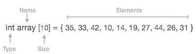
Arrays can be declared in various ways in different languages. For illustration, let's take C array declaration.

As per the above illustration, following are the important points to be considered.

• Index starts with 0.
• Array length is 10 which means it can store 10 elements.
• Each element can be accessed via its index. For example, we can fetch an element at index 6 as 9.
• 
  

Basic Operations

Following are the basic operations supported by an array.

• Traverse − print all the array elements one by one.
• Insertion − Adds an element at the given index.
• Deletion − Deletes an element at the given index.
• Search − Searches an element using the given index or by the value.
• Update − Updates an element at the given index.

In C, when an array is initialized with size, then it assigns defaults values to its elements in following order.

Data Type	Default Value
bool	false
char	0
int	0
float	0.0
double	0.0f
void
wchar_t	0

Insertion Operation

Insert operation is to insert one or more data elements into an array. Based on the requirement, a new element can be added at the beginning, end, or any given index of array.

Here, we see a practical implementation of insertion operation, where we add data at the end of the array −

Algorithm

Let Array be a linear unordered array of MAX elements.

Example

Result

Let LA be a Linear Array (unordered) with N elements and K is a positive integer such that K<=N. Following is the algorithm where ITEM is inserted into the K^th position of LA −

1. Start
2. Set J = N
3. Set N = N+1
4. Repeat steps 5 and 6 while J >= K
5. Set LA[J+1] = LA[J]
6. Set J = J-1
7. Set LA[K] = ITEM
8. Stop

Example

Following is the implementation of the above algorithm −

#include <stdio.h>

main() {
   int LA[] = {1,3,5,7,8};
   int item = 10, k = 3, n = 5;
   int i = 0, j = n;
   
   printf("The original array elements are :\n");

   for(i = 0; i<n; i++) {
      printf("LA[%d] = %d \n", i, LA[i]);
   }

   n = n + 1;
 
   while( j >= k) {
      LA[j+1] = LA[j];
      j = j - 1;
   }

   LA[k] = item;

   printf("The array elements after insertion :\n");

   for(i = 0; i<n; i++) {
      printf("LA[%d] = %d \n", i, LA[i]);
   }
}

When we compile and execute the above program, it produces the following result −

Output

The original array elements are :
LA[0] = 1 
LA[1] = 3 
LA[2] = 5 
LA[3] = 7 
LA[4] = 8 
The array elements after insertion :
LA[0] = 1 
LA[1] = 3 
LA[2] = 5 
LA[3] = 10 
LA[4] = 7 
LA[5] = 8 

For other variations of array insertion operation click here

Deletion Operation

Deletion refers to removing an existing element from the array and re-organizing all elements of an array.

Algorithm

Consider LA is a linear array with N elements and K is a positive integer such that K<=N. Following is the algorithm to delete an element available at the K^th position of LA.

1. Start
2. Set J = K
3. Repeat steps 4 and 5 while J < N
4. Set LA[J] = LA[J + 1]
5. Set J = J+1
6. Set N = N-1
7. Stop

Example

Following is the implementation of the above algorithm −

#include <stdio.h>

void main() {
   int LA[] = {1,3,5,7,8};
   int k = 3, n = 5;
   int i, j;
   
   printf("The original array elements are :\n");
 
   for(i = 0; i<n; i++) {
      printf("LA[%d] = %d \n", i, LA[i]);
   }
    
   j = k;
 
   while( j < n) {
      LA[j-1] = LA[j];
      j = j + 1;
   }
 
   n = n -1;
   
   printf("The array elements after deletion :\n");
 
   for(i = 0; i<n; i++) {
      printf("LA[%d] = %d \n", i, LA[i]);
   }
}

When we compile and execute the above program, it produces the following result −

Output

The original array elements are :
LA[0] = 1 
LA[1] = 3 
LA[2] = 5 
LA[3] = 7 
LA[4] = 8 
The array elements after deletion :
LA[0] = 1 
LA[1] = 3 
LA[2] = 7 
LA[3] = 8 

Search Operation

You can perform a search for an array element based on its value or its index.

Algorithm

Consider LA is a linear array with N elements and K is a positive integer such that K<=N. Following is the algorithm to find an element with a value of ITEM using sequential search.

1. Start
2. Set J = 0
3. Repeat steps 4 and 5 while J < N
4. IF LA[J] is equal ITEM THEN GOTO STEP 6
5. Set J = J +1
6. PRINT J, ITEM
7. Stop

Example

Following is the implementation of the above algorithm −

#include <stdio.h>

void main() {
   int LA[] = {1,3,5,7,8};
   int item = 5, n = 5;
   int i = 0, j = 0;
   
   printf("The original array elements are :\n");
 
   for(i = 0; i<n; i++) {
      printf("LA[%d] = %d \n", i, LA[i]);
   }
    
   while( j < n){
      if( LA[j] == item ) {
         break;
      }
  
      j = j + 1;
   }
 
   printf("Found element %d at position %d\n", item, j+1);
}

When we compile and execute the above program, it produces the following result −

Output

The original array elements are :
LA[0] = 1 
LA[1] = 3 
LA[2] = 5 
LA[3] = 7 
LA[4] = 8 
Found element 5 at position 3

Update Operation

Update operation refers to updating an existing element from the array at a given index.

Algorithm

Consider LA is a linear array with N elements and K is a positive integer such that K<=N. Following is the algorithm to update an element available at the K^th position of LA.

1. Start
2. Set LA[K-1] = ITEM
3. Stop

Example

Following is the implementation of the above algorithm −

#include <stdio.h>

void main() {
   int LA[] = {1,3,5,7,8};
   int k = 3, n = 5, item = 10;
   int i, j;
   
   printf("The original array elements are :\n");
 
   for(i = 0; i<n; i++) {
      printf("LA[%d] = %d \n", i, LA[i]);
   }
    
   LA[k-1] = item;

   printf("The array elements after updation :\n");
 
   for(i = 0; i<n; i++) {
      printf("LA[%d] = %d \n", i, LA[i]);
   }
}

When we compile and execute the above program, it produces the following result −

Output

The original array elements are :
LA[0] = 1 
LA[1] = 3 
LA[2] = 5 
LA[3] = 7 
LA[4] = 8 
The array elements after updation :
LA[0] = 1 
LA[1] = 3 
LA[2] = 10 
LA[3] = 7 
LA[4] = 8