Basics of Data Structures and Algorithms

Algorithm is a step-by-step procedure, which defines a set of instructions to be executed in a certain order to get the desired output. Algorithms are generally created independent of underlying languages, i.e. an algorithm can be implemented in more than one programming language.

From the data structure point of view, following are some important categories of algorithms −

· Search − Algorithm to search an item in a data structure.

· Sort − Algorithm to sort items in a certain order.

· Insert − Algorithm to insert item in a data structure.

· Update − Algorithm to update an existing item in a data structure.

· Delete − Algorithm to delete an existing item from a data structure.

Characteristics of an Algorithm

Not all procedures can be called an algorithm. An algorithm should have the following characteristics −

· Unambiguous − Algorithm should be clear and unambiguous. Each of its steps (or phases), and their inputs/outputs should be clear and must lead to only one meaning.

· Input − An algorithm should have 0 or more well-defined inputs.

· Output − An algorithm should have 1 or more well-defined outputs, and should match the desired output.

· Finiteness − Algorithms must terminate after a finite number of steps.

· Feasibility − Should be feasible with the available resources.

· Independent − An algorithm should have step-by-step directions, which should be independent of any programming code.

How to Write an Algorithm?

There are no well-defined standards for writing algorithms. Rather, it is problem and resource dependent. Algorithms are never written to support a particular programming code.

As we know that all programming languages share basic code constructs like loops (do, for, while), flow-control (if-else), etc. These common constructs can be used to write an algorithm.

We write algorithms in a step-by-step manner, but it is not always the case. Algorithm writing is a process and is executed after the problem domain is well-defined. That is, we should know the problem domain, for which we are designing a solution.

Example

Let's try to learn algorithm-writing by using an example.

Problem − Design an algorithm to add two numbers and display the result.

Step 1 − START

Step 2 − declare three integers a, b & c

Step 3 − define values of a & b

Step 4 − add values of a & b

Step 5 − store output of step 4 to c

Step 6 − print c

Step 7 − STOP

Algorithms tell the programmers how to code the program. Alternatively, the algorithm can be written as −

Step 1 − START ADD

Step 2 − get values of a & b

Step 3 − c ← a + b

Step 4 − display c

Step 5 − STOP

In design and analysis of algorithms, usually the second method is used to describe an algorithm. It makes it easy for the analyst to analyze the algorithm ignoring all unwanted definitions. He can observe what operations are being used and how the process is flowing.

Writing step numbers, is optional.

We design an algorithm to get a solution of a given problem. A problem can be solved in more than one ways.

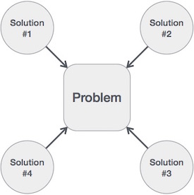
Hence, many solution algorithms can be derived for a given problem. The next step is to analyze those proposed solution algorithms and implement the best suitable solution.

Algorithm Analysis

Efficiency of an algorithm can be analyzed at two different stages, before implementation and after implementation. They are the following −

· A Priori Analysis − This is a theoretical analysis of an algorithm. Efficiency of an algorithm is measured by assuming that all other factors, for example, processor speed, are constant and have no effect on the implementation.

· A Posterior Analysis − This is an empirical analysis of an algorithm. The selected algorithm is implemented using programming language. This is then executed on target computer machine. In this analysis, actual statistics like running time and space required, are collected.

We shall learn about a priori algorithm analysis. Algorithm analysis deals with the execution or running time of various operations involved. The running time of an operation can be defined as the number of computer instructions executed per operation.

Algorithm Complexity

Suppose X is an algorithm and n is the size of input data, the time and space used by the algorithm X are the two main factors, which decide the efficiency of X.

· Time Factor − Time is measured by counting the number of key operations such as comparisons in the sorting algorithm.

· Space Factor − Space is measured by counting the maximum memory space required by the algorithm.

The complexity of an algorithm f(n) gives the running time and/or the storage space required by the algorithm in terms of n as the size of input data.

Space Complexity

Space complexity of an algorithm represents the amount of memory space required by the algorithm in its life cycle. The space required by an algorithm is equal to the sum of the following two components −

· A fixed part that is a space required to store certain data and variables, that are independent of the size of the problem. For example, simple variables and constants used, program size, etc.

· A variable part is a space required by variables, whose size depends on the size of the problem. For example, dynamic memory allocation, recursion stack space, etc.

Space complexity S(P) of any algorithm P is S(P) = C + SP(I), where C is the fixed part and S(I) is the variable part of the algorithm, which depends on instance characteristic I. Following is a simple example that tries to explain the concept −

Algorithm: SUM(A, B)

Step 1 - START

Step 2 - C ← A + B + 10

Step 3 - Stop

Here we have three variables A, B, and C and one constant. Hence S(P) = 1 + 3. Now, space depends on data types of given variables and constant types and it will be multiplied accordingly.

Time Complexity

Time complexity of an algorithm represents the amount of time required by the algorithm to run to completion. Time requirements can be defined as a numerical function T(n), where T(n) can be measured as the number of steps, provided each step consumes constant time.

For example, addition of two n-bit integers takes n steps. Consequently, the total computational time is T(n) = c ∗ n, where c is the time taken for the addition of two bits. Here, we observe that T(n) grows linearly as the input size increases.

Comments

Digital Signal Processing - Basic Continuous Time Signals

To test a system, generally, standard or basic signals are used. These signals are the basic building blocks for many complex signals. Hence, they play a very important role in the study of signals and systems. Unit Impulse or Delta Function A signal, which satisfies the condition, δ ( t ) = lim ϵ → ∞ x ( t ) δ ( t ) = lim ϵ → ∞ x ( t ) is known as unit impulse signal. This signal tends to infinity when t = 0 and tends to zero when t ≠ 0 such that the area under its curve is always equals to one. The delta function has zero amplitude everywhere except at t = 0. Properties of Unit Impulse Signal δ(t) is an even signal. δ(t) is an example of neither energy nor power (NENP) signal. Area of unit impulse signal can be written as; A = ∫ ∞ − ∞ δ ( t ) d t = ∫ ∞ − ∞ lim ϵ → 0 x ( t ) d t = lim ϵ → 0 ∫ ∞ − ∞ [ x ( t ) d t ] = 1 Weight or strength of the signal can be written as; y ( t ) = A δ ( t ) y ( t ) = A δ ( t ) Area of the weighted impulse s...

Differential Equations - First Order: Bernoulli

In this section we are going to take a look at differential equations in the form, y ′ + p ( x ) y = q ( x ) y n y ′ + p ( x ) y = q ( x ) y n where p ( x ) p ( x ) and q ( x ) q ( x ) are continuous functions on the interval we’re working on and n n is a real number. Differential equations in this form are called Bernoulli Equations . First notice that if n = 0 n = 0 or n = 1 n = 1 then the equation is linear and we already know how to solve it in these cases. Therefore, in this section we’re going to be looking at solutions for values of n n other than these two. In order to solve these we’ll first divide the differential equation by y n y n to get, y − n y ′ + p ( x ) y 1 − n = q ( x ) y − n y ′ + p ( x ) y 1 − n = q ( x ) We are now going to use the substitution v = y 1 − n v = y 1 − n to convert this into a differential equation in terms of v v . As we’ll see th...

Differential Equations - Systems: Solutions

Now that we’ve got some of the basics out of the way for systems of differential equations it’s time to start thinking about how to solve a system of differential equations. We will start with the homogeneous system written in matrix form, → x ′ = A → x (1) (1) x → ′ = A x → where, A A is an n × n n × n matrix and → x x → is a vector whose components are the unknown functions in the system. Now, if we start with n = 1 n = 1 then the system reduces to a fairly simple linear (or separable) first order differential equation. x ′ = a x x ′ = a x and this has the following solution, x ( t ) = c e a t x ( t ) = c e a t So, let’s use this as a guide and for a general n n let’s see if → x ( t ) = → η e r t (2) (2) x → ( t ) = η → e r t will be a solution. Note that the only real difference here is that we let the constant in front of the exponential be a vector. All we need to do then is plug this into the d...

Digital Signal Processing - Miscellaneous Signals

There are other signals, which are a result of operation performed on them. Some common type of signals are discussed below. Conjugate Signals Signals, which satisfies the condition x ( t ) = x ∗ ( − t ) are called conjugate signals. Let x ( t ) = a ( t ) + j b ( t ) So, x ( − t ) = a ( − t ) + j b ( − t ) And x ∗ ( − t ) = a ( − t ) − j b ( − t ) By Condition, x ( t ) = x ∗ ( − t ) If we compare both the derived equations 1 and 2, we can see that the real part is even, whereas the imaginary part is odd. This is the condition for a signal to be a conjugate type. Conjugate Anti-Symmetric Signals Signals, which satisfy the condition x ( t ) = − x ∗ ( − t ) are called conjugate anti-symmetric signal Let x ( t ) = a ( t ) + j b ( t ) So x ( − t ) = a ( − t ) + j b ( − t ) And x ∗ ( − t ) = a ( − t ) − j b ( − t ) − x ∗ ( − t ) = − a ( − t ) + j b ( − t ) By Condition x ( t ) = − x ∗ ( − t ) ...

Calculus III - 3-Dimensional Space: Equations of Lines

In this section we need to take a look at the equation of a line in R 3 R 3 . As we saw in the previous section the equation y = m x + b y = m x + b does not describe a line in R 3 R 3 , instead it describes a plane. This doesn’t mean however that we can’t write down an equation for a line in 3-D space. We’re just going to need a new way of writing down the equation of a curve. So, before we get into the equations of lines we first need to briefly look at vector functions. We’re going to take a more in depth look at vector functions later. At this point all that we need to worry about is notational issues and how they can be used to give the equation of a curve. The best way to get an idea of what a vector function is and what its graph looks like is to look at an example. So, consider the following vector function. → r ( t ) = ⟨ t , 1 ⟩ r → ( t ) = ⟨ t , 1 ⟩ A vector function is a function that takes one or more variables, one in this case, and returns a...

Differential Equations - First Order: Modeling - i

We now move into one of the main applications of differential equations both in this class and in general. Modeling is the process of writing a differential equation to describe a physical situation. Almost all of the differential equations that you will use in your job (for the engineers out there in the audience) are there because somebody, at some time, modeled a situation to come up with the differential equation that you are using. This section is not intended to completely teach you how to go about modeling all physical situations. A whole course could be devoted to the subject of modeling and still not cover everything! This section is designed to introduce you to the process of modeling and show you what is involved in modeling. We will look at three different situations in this section : Mixing Problems, Population Problems, and Falling Objects. In all of these situations we will be forced to make assumptions that do not accurately depict reality in most cases, but wi...

Differential Equations - Basic Concepts: Definitions

Differential Equation The first definition that we should cover should be that of differential equation . A differential equation is any equation which contains derivatives, either ordinary derivatives or partial derivatives. There is one differential equation that everybody probably knows, that is Newton’s Second Law of Motion. If an object of mass m m is moving with acceleration a a and being acted on with force F F then Newton’s Second Law tells us. F = m a (1) (1) F = m a To see that this is in fact a differential equation we need to rewrite it a little. First, remember that we can rewrite the acceleration, a a , in one of two ways. a = d v d t OR a = d 2 u d t 2 (2) (2) a = d v d t OR a = d 2 u d t 2 Where v v is the velocity of the object and u u is the position function of the object at any time t t . We should also remember at this point that the force, F F may also be a f...

Differential Equations - Second Order: Repeated Roots

In this section we will be looking at the last case for the constant coefficient, linear, homogeneous second order differential equations. In this case we want solutions to a y ′′ + b y ′ + c y = 0 a y ″ + b y ′ + c y = 0 where solutions to the characteristic equation a r 2 + b r + c = 0 a r 2 + b r + c = 0 are double roots r 1 = r 2 = r r 1 = r 2 = r . This leads to a problem however. Recall that the solutions are y 1 ( t ) = e r 1 t = e r t y 2 ( t ) = e r 2 t = e r t y 1 ( t ) = e r 1 t = e r t y 2 ( t ) = e r 2 t = e r t These are the same solution and will NOT be “nice enough” to form a general solution. We do promise that we’ll define “nice enough” eventually! So, we can use the first solution, but we’re going to need a second solution. Before finding this second solution let’s take a little side trip. The reason for the side trip will be clear eventually. From the quadratic formula we know that the roots to the characteristic equation are, r 1 , 2 = ...

Differential Equations - Systems: Repeated Eigenvalues - i

This is the final case that we need to take a look at. In this section we are going to look at solutions to the system, → x ′ = A → x x → ′ = A x → where the eigenvalues are repeated eigenvalues. Since we are going to be working with systems in which A A is a 2 × 2 2 × 2 matrix we will make that assumption from the start. So, the system will have a double eigenvalue, λ λ . This presents us with a problem. We want two linearly independent solutions so that we can form a general solution. However, with a double eigenvalue we will have only one, → x 1 = → η e λ t x → 1 = η → e λ t So, we need to come up with a second solution. Recall that when we looked at the double root case with the second order differential equations we ran into a similar problem. In that section we simply added a t t to the solution and were able to get a second solution. Let’s see if the same thing will work in this case as well. We’ll see if → x = t e...

Differential Equations - Partial: Summary of Separation of Variables

Throughout this chapter we’ve been talking about and solving partial differential equations using the method of separation of variables. However, the one thing that we’ve not really done is completely work an example from start to finish showing each and every step. Each partial differential equation that we solved made use somewhere of the fact that we’d done at least part of the problem in another section and so it makes some sense to have a quick summary of the method here. Also note that each of the partial differential equations only involved two variables. The method can often be extended out to more than two variables, but the work in those problems can be quite involved and so we didn’t cover any of that here. So with all of that out of the way here is a quick summary of the method of separation of variables for partial differential equations in two variables. Verify that the partial differential equation is linear and homogeneous. Verify that the boundary condi...

Robert Karamagi

Search This Blog

Calculus III - 3-Dimensional Space: Equations of Lines